Mirror Descent and Bregman Divergences
16 November 2026
When optimising a differentiable function $f: X \to \R$ over a (possibly constrained) set $X \subseteq \R^d$, our go-to algorithm is gradient descent
\[x_{t+1} = x_t - \eta \nabla f(x_t),\]followed by a projection onto $X$ when $X$ is constrained. Completing the square, this projected gradient step can equivalently be written as the proximal update
\[x_{t+1} = \argmin_{x \in X} \left\{ \langle x, \nabla f(x_t) \rangle + \frac{1}{2\eta} \lVert x - x_t \rVert^2 \right\}.\]Here, $x \mapsto \langle x, \nabla f(x_t) \rangle$ is, up to an additive constant, the linearisation of $f$ around $x_t$. The term $\frac{1}{2\eta}\lVert x - x_t \rVert^2$ is a penalty keeping us close to $x_t$, since we only trust the linear approximation locally.
The thing to notice is that this penalty implicitly equips $X$ with the Euclidean geometry, which can be a poor notion of “nearness”. For example, if $X = \Delta_d \subseteq \R^d$ is the probability simplex, changing the probability of an event from $0.001$ to $0.002$ is significant (it doubles), whereas changing it from $0.501$ to $0.502$ is not; yet the Euclidean distance treats these equally. Algorithms that ignore the geometry of $X$ in this way can perform poorly in practice. Moreover, when $X$ is constrained, simply projecting back onto $X$ (as in projected gradient descent) can be problematic.
The basic idea of mirror descent is to replace the squared Euclidean distance with a Bregman divergence. This allows the update to adapt to non-Euclidean geometries and, in particular, to handle constraints naturally.
Bregman Divergences
At an intuitive level, Bregman divergences generalise the squared Euclidean distance. Let $\phi: X \to \R$ be differentiable and strictly convex. Its associated Bregman divergence is
\[D_\phi(x, y) = \phi(x) - \phi(y) - \langle \nabla \phi(y), x - y \rangle.\]Geometrically, this is the gap at $x$ between $\phi$ and its linearisation around $y$. By strict convexity, $D_\phi(x, y) \geq 0$ with equality iff $x = y$. However, $D_\phi$ is generally asymmetric and does not satisfy the triangle inequality, so it is not a metric.
Two standard examples:
- For the quadratic energy $\phi(x) = \frac{1}{2}\lVert x \rVert^2$, we recover $D_\phi(x,y) = \frac{1}{2} \lVert x - y \rVert^2$.
- If $X = \Delta_d$ and $\phi(x) = \sum_{i=1}^d x_i \log x_i$ is the negative Shannon entropy, then, using $\sum_i x_i = \sum_i y_i = 1$, we get $D_\phi(x, y) = \sum_i x_i \log(x_i / y_i) = {\sf KL}[x \,\Vert\, y]$.
Mirror Descent
In mirror descent, one replaces the Euclidean penalty in the proximal update with a Bregman divergence:
\[x_{t+1} = \argmin_{x \in X} \left\{ \langle x, \nabla f(x_t) \rangle + \frac{1}{\eta} D_\phi(x, x_t) \right\}. \tag{MD}\]Setting the gradient of the objective to zero gives $\nabla f(x_t) + \frac{1}{\eta}\left(\nabla \phi(x_{t+1}) - \nabla \phi(x_t)\right) = 0$, i.e.,
\[\nabla \phi (x_{t+1}) = \nabla \phi (x_t) - \eta \nabla f(x_t).\]This is exact when $x_{t+1}$ lies in the interior of $X$. In general, the optimality condition only holds up to an element of the normal cone of $X$ at $x_{t+1}$; for the simplex, this is a multiple of $\mathbf{1}$, which is absorbed by normalisation (see the example below).
We see that this is ordinary gradient descent, except that it acts on $\nabla \phi(x_t)$, i.e., after mapping a point $x_t$ into the dual space. To recover $x_{t+1}$, we need the inverse map $(\nabla \phi)^{-1}$.
This is exactly what convex conjugates provide. Recall that the convex conjugate of $\phi$ is the map $\phi^\ast: \R^d \to \R \cup \lbrace +\infty \rbrace$ defined by
\[\phi^*(y) = \sup_{x \in X} \{ \langle x, y \rangle - \phi(x) \}.\]Note that $\phi^\ast$ takes slopes $y$ as input, and these live in the dual space $\R^d$ rather than in $X$. For sufficiently nice $\phi$ (e.g. of Legendre type; see Rockafellar, 1970, Theorems 23.5 and 26.5), we have
\[y = \nabla \phi(x) \iff x = \nabla \phi^*(y) \iff \phi(x) + \phi^*(y) = \langle x, y \rangle.\]Hence $(\nabla \phi)^{-1} = \nabla \phi^\ast$. The heuristic is that the conjugate reparametrises $\phi$ in terms of its slopes: $\nabla \phi$ gives the slope at a point, and $\nabla \phi^\ast$ gives the point with a given slope.
Consequently, a mirror descent step can be implemented as follows:
- Map $x_t$ to the dual space via $\nabla \phi$.
- Take an ordinary gradient step there, using $\nabla f(x_t)$.
- Map back to $X$ via $\nabla \phi^\ast$.
That is,
\[x_{t+1} = \nabla \phi^* \left(\nabla \phi (x_t) - \eta \nabla f (x_t)\right).\]This requires $\nabla \phi$ and $\nabla \phi^\ast$ to be cheap to evaluate.
Take $X = \Delta_d$ and $\phi(x) = \sum_{i=1}^d x_i \log x_i$, so that $D_\phi$ is the KL divergence. Rather than computing $\phi^\ast$, we can solve (MD) directly with a Lagrange multiplier $\lambda$ for the constraint $\sum_i x_i = 1$. Stationarity in $x_i$ gives
\[(\nabla f(x_t))_i + \frac{1}{\eta}\left(\log \frac{x_i}{x_{t,i}} + 1\right) + \lambda = 0,\]so $x_i \propto x_{t,i} \exp(-\eta (\nabla f(x_t))_i)$; the nonnegativity constraints are inactive. Normalising yields
\[x_{t+1,i} = \frac{x_{t,i} \exp(-\eta (\nabla f(x_t))_i)}{\sum_j x_{t,j} \exp(-\eta (\nabla f(x_t))_j)}.\]This is a multiplicative re-weighting of $x_t$, which stays in $\Delta_d$ automatically, so no projection is needed.
The mirror map is $\nabla \phi(x) = \mathbf{1} + \log x$ (componentwise), which maps into the logits up to an additive constant. The conjugate is the log-sum-exp function $\phi^\ast(y) = \log \sum_i \exp(y_i)$, whose gradient $\nabla \phi^\ast$ is the softmax. Indeed, applying the softmax to $\nabla \phi(x_t) - \eta \nabla f(x_t)$ recovers the update above, so entropic mirror descent is an additive update on the logits.
Why Bregman Divergences?
It seems we could have used any distance-like penalty in the proximal update. Why use Bregman divergences in particular?
First, the Bregman form is exactly what leads to the closed-form “gradient step in the dual” update. Expanding the definition, $D_\phi(x, x_t) = \phi(x) - \langle \nabla \phi(x_t), x \rangle + C$, where $C$ does not depend on $x$. Hence the objective in (MD) is
\[\langle x, \nabla f(x_t) \rangle + \frac{1}{\eta}D_\phi(x, x_t) = \frac{1}{\eta} \left( \phi(x) - \langle \nabla \phi(x_t) - \eta \nabla f (x_t), x \rangle \right) + \frac{C}{\eta},\]so the linear part of $D_\phi$ combines with $\nabla f(x_t)$. Minimising this over $x \in X$ is exactly the maximisation defining $\phi^\ast$ at $\nabla \phi(x_t) - \eta \nabla f(x_t)$, whose maximiser is $\nabla \phi^\ast(\nabla \phi(x_t) - \eta \nabla f(x_t))$ (Rockafellar, 1970, Theorem 23.5). This recovers the mirror descent update directly, with no interiority assumption. A generic distance-like penalty lacks this structure, and the proximal step is then an arbitrary nonlinear optimisation problem.
Second, Bregman divergences retain enough structure for analyses to remain tractable. In particular, expanding the definitions gives the three-point identity
\[D_\phi(x, y) + D_\phi(y, z) - D_\phi(x, z) = \langle \nabla \phi (z) - \nabla \phi(y), x - y \rangle.\]For $\phi = \frac{1}{2}\lVert \cdot \rVert^2$, this is the law of cosines. It plays the same role in convergence proofs, making sums of divergences telescope despite the lack of symmetry and the triangle inequality.
Bregman Geometry
In fact, the dichotomy of “Bregman divergence versus squared distance” is a false one. Locally, Bregman divergences are half squared distances, so choosing a Bregman divergence implicitly selects a geometry to work in. Since the proximal update is local, this is all that matters. To see this, we study some differential-geometric aspects of Bregman divergences.
Assume $\phi$ is smooth, and let $H(x) = \nabla^2 \phi(x)$ and $T(x) = \nabla^3 \phi(x)$ be its second and third derivatives. A Taylor expansion around $x$ yields
\[\phi(x+v) = \phi(x) + v^{\top} \nabla \phi(x) + \frac{1}{2} v^{\top} H(x) v + \frac{1}{6} T(x)[v, v, v] + O(\lVert v \rVert^4),\]so that
\[D_\phi(x+v, x) = \frac{1}{2} v^{\top} H(x) v + \frac{1}{6} T(x)[v,v,v] + O(\lVert v \rVert^4).\]Similarly, since $\langle \nabla \phi(x+ v), v \rangle = v^{\top} \nabla \phi(x) + v^{\top }H(x) v + \frac{1}{2}T(x)[v,v,v] + O(\lVert v \rVert^4)$, the reverse divergence is
\[D_\phi(x, x+v) = \frac{1}{2} v^{\top} H(x) v + \frac{1}{3} T(x)[v,v,v] + O(\lVert v \rVert^4).\]Hence, to second order, $D_\phi$ is symmetric and equal to the quadratic form $\frac{1}{2} v^{\top} H(x) v$; the asymmetry only enters at third order, through $T$.
Suppose further that $H(x)$ is positive definite; strict convexity alone does not guarantee this (consider $\phi(x) = x^4$ at $0$). Then $\langle u, w \rangle_x = u^{\top} H(x) w$ defines a Riemannian metric, which we call the Hessian metric of $\phi$. If $d_H$ is the corresponding geodesic distance, then $d_H(x, x+v)^2 = v^{\top} H(x) v + O(\lVert v \rVert^3)$, and so
\[D_\phi(x+v, x) = \frac{1}{2} d_H(x, x+v)^2 + O(\lVert v \rVert^3).\]This makes precise the sense in which Bregman divergences behave like squared distances.
Let $X = \Delta_d$ and $\phi(x) = \sum_i x_i \log x_i$, so that $D_\phi(x, y) = {\sf KL}[x \,\Vert\, y]$. The Hessian is $\nabla^2 \phi(x) = \mathrm{diag}(1/x_i)$, which, on tangent vectors $v$ with $\sum_i v_i = 0$, is exactly the Fisher information metric of the categorical family. The corresponding geodesic distance is the Fisher-Rao distance $d_{\mathrm{FR}}(x,y) = 2 \arccos \left( \langle \sqrt{x}, \sqrt{y} \rangle \right)$, with the square root taken componentwise. We thus see
\[{\sf KL}[x + v \,\Vert\, x] \approx \frac{1}{2} \sum_i \frac{v_i^2}{x_i} \approx \frac{1}{2} d_{\mathrm{FR}}(x + v, x)^2,\]where the middle term is half the $\chi^2$ divergence of $x + v$ from $x$.
In short, the KL divergence is, to second order, half the squared Fisher-Rao distance: entropic mirror descent implicitly works in the Fisher-Rao geometry.
The Continuous-Time Limit
Mirror descent is a discrete-time algorithm, and we can informally derive its continuous-time limit. Rearranging the update gives
\[\frac{\nabla \phi(x_{t+1}) - \nabla \phi(x_t)}{\eta} = - \nabla f(x_t).\]Interpreting $\eta$ as a time step and letting $\eta \to 0$, we obtain the ODE
\[\frac{\d}{\d t} \nabla \phi(x_t) = - \nabla f(x_t).\]By the chain rule, the left-hand side is $H(x_t) \frac{\d}{\d t} x_t$, so in the primal space this reads
\[\frac{\d}{\d t} x_t = - H(x_t)^{-1} \nabla f(x_t).\]Here $H(x_t)^{-1} \nabla f(x_t)$ is precisely the Riemannian gradient of $f$ under the Hessian metric. Thus, mirror descent is a time-discretisation of the Riemannian gradient flow of $f$ under the geometry induced by $\phi$. More precisely, it is the forward Euler scheme for these dynamics, written in the dual coordinates $\nabla \phi(x_t)$.
Summary
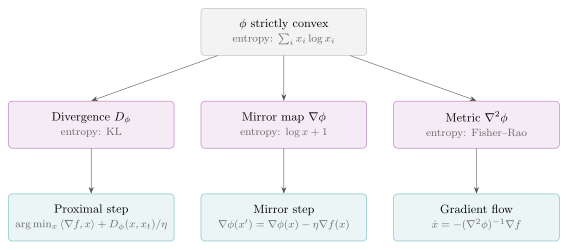
Starting from the problem of optimising $f$ over a constrained set or a non-Euclidean space, we generalised the proximal form of gradient descent by replacing the squared Euclidean distance with a Bregman divergence. Convex duality shows that the resulting update is a gradient step in the dual space, implemented via the mirror map $\nabla \phi$ and its inverse $\nabla \phi^\ast$. Differential geometry shows that the Bregman divergence is locally a half squared distance under the Hessian metric of $\phi$, and that mirror descent is a forward Euler discretisation of the corresponding Riemannian gradient flow. These connections are summarised in the figure below.
References.
- Nemirovski, A. and Yudin, D. (1983). Problem Complexity and Method Efficiency in Optimization.
- Beck, A. and Teboulle, M. (2003). Mirror descent and nonlinear projected subgradient methods for convex optimization. Operations Research Letters.
- Rockafellar, R. T. (1970). Convex Analysis, Sections 23 and 26.